Getting Started with the AKD/AKD2G Performance Tuner (PST)

This document reviews the basics of getting started with the PST (Performance Servo Tuner). There are several references in this document to other documents for more detailed information.  

The Workbench PST can fully tune the drive for your application by automatically determining the  servo gains and filter parameters.

 

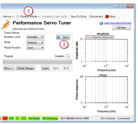
1. Running the Workbench PST (Performance Servo Tuner)

The PST collects frequency response data (bode plot) that can be used for advanced analysis.

Tuning settings to start:

       

Set opmode to: Position

          

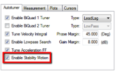
Load Position when running the PST: The axis position should not be placed near the end of travel, as this could adversely affect the results.  There is some movement of the motor during the test. At the end of the test if Enable Stable Motion is selected to verify performance, the motor will additionally move ½ rev CW then CCW. If not selected the motor will have a maximum movement of +/- 1/8 motor rev.

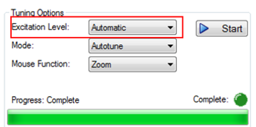
Running the PST: Click on the Start button to run through a series of test to determine friction, verify direction, and then excite the motor with a series of frequencies

After completed new tuning values are set you and you can test the results (in the time domain) by executing motion with the WorkBench scope or  the  motion controller on the machine.  If machine performance is satisfactory, you are finished and can save the new  tuning values to the drives non-volatile memory.

The PST will attempt to tune your system to a high BW, GM (Gain Margin) = 8 dB and PM(Phase Margin) = 45 degrees which may be too high (very stiff and possibly audibly noisy)for your application. If this is the case the margins can be raised  Example: set GM (Gain Margin) = 10 dB and PM(Phase Margin) = 55 degrees. The result may then be acceptable performance with a  lower BW which could result in lower  audible noise and be softer on the system mechanics.

 

2. System Performance

a. Analyzing the Bode Plot

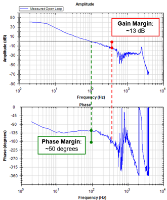
First verify a good plot has been created by the PST. The PST  creates a Bode Plot which can be read to determines performance in terms of BW(bandwidth), Phase Margin(PM) and Gain Margin (GM). See article: Bode plot Interpretation and Use

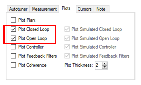
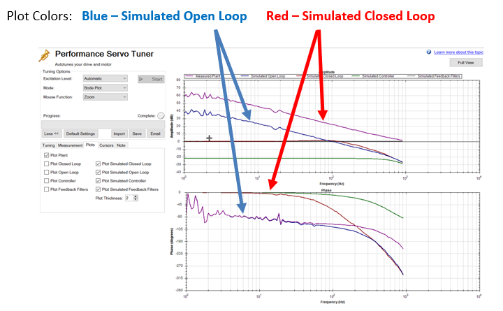
Plot Colors:   Blue – Open Loop      Red – Closed Loop

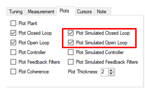
To get a clear view on the plot check only the “Plot close loop” and “Plot open loop” boxes as follows:

   

Key attributes of a good  bode plot in which performance can be calculated are:

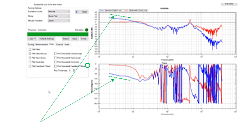
• The open loop (blue plot)  phase (going left to right) starts out at -90 degrees and has a magnitude slope of -20dB/decade.
• If the open loop (blue plot)  phase (going left to right) ramps upward as oppose to ramping downward  the plot is not good, very likely due to friction, backlash, or a very large load.

An optimum plot that provides acceptable servo performance with most loads has the following attributes:

• The 2 bullets above that make a useable plot
• The close loop gain is never greater than + 3dB  at frequencies within the system BW and never greater than 0 dB at frequencies greater than the system BW
• The open loop crossover occurs at or near the closed loop BW.
• Phase Margin is 45 degr and Gain Margin is 8 dB or greater. For many mechanics with low compliance these margins can be less. Occasionally the values may need to be higher for high compliance system especially with large inertias.
• Example: good bode plot with good servo performance:

 

b. Analyzing the Bode Plot

1. If the plot does is not usable, adjustments can be made to the commands within the PST. To make the adjustments, change the excitation level to Manual and go to the Measurement sub tab

 

 

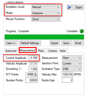
            Increase the current amplitude. This can often be required to overcome friction or to have enough current for larger inertia loads.

• Example plot of friction at low frequencies in a complex load with multiple resonance points:

      

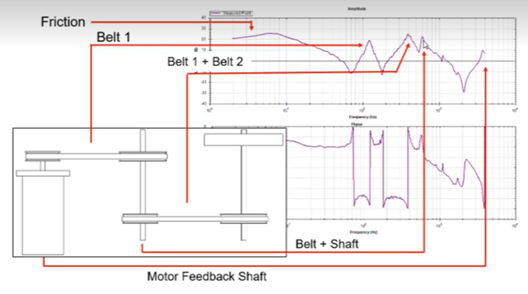
Change excitation type.  By default, the PST  will excite the system with Pseudo Random Binary Bit Toggle, called PRB. There are 2 alternative excitation methods: sine wave and a noise excitation signal.

            

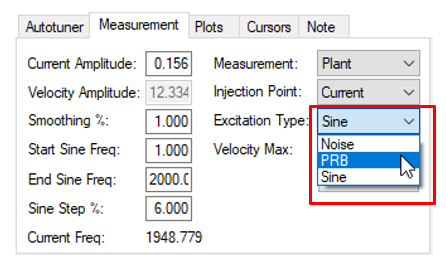
             Each one has a unique input but will analyze the signal the same way. The noise excitation is the simultaneous excitation of all the frequencies simultaneously not unlike FM noise on radio signals and the PRB (default) is essentially a repeating square wave input to the drive. In most cases, PRB (the default method) may be the easiest implementation with l                 ittle movement in the system but have good low frequency response.        

             Summary – which Excitation Type to use:                    

Type	When to use	Movement
PRB - default	The default (can be used in most applications)	The signal varies between +/- current or velocity amplitude (depending on injection point). Minimal typically within +1/4 rev if “Enable Stability Motion “ box not checked, +1/2 rev if checked
Noise	If you have an actual load instability that does not show up on the bode plot, noise excitation provides more frequency data on the input to the plant.	The signal varies between +/- current or velocity amplitude (depending on injection point). Minimal typically within +1/4 rev if “Enable Stability Motion “ box not checked, +1/2 rev if checked
Sine - Take longer to run but provides more information to the PST.  Only use if the system can allow reciprocating motion. Typically used on very large loads.	Good to use in Low BW , large inertia, or highly compliant load. Sinewave excitation: requires that you specify the start frequency, end frequency, and frequency step size. The sine sweep takes significantly longer than a noise or PRB measurement but is often cleaner. Be careful when selecting a step size: too large of a step size may miss important resonances, and too small of a step size increases measurement time.	+/- 2 revs or less depending on the system including motor size. Do not use in applications that cannot move bidirectionally

 

            Change to Velocity Cmd (from Current Cmd)

           In closed loop applications, it is sometimes desirable to use a velocity excitation to the loop to see  stable  measurements. The difference with  inputting velocity as opposed to current is that you are not looking at the Plant but looking for how the system reacts  to the velocity input including all filtering. In Plant measurements, the input is not affected by                   the  closed loop gains.

For more information on understanding Bode plots:

• link to article Using Bode Plots to Improve Performance
• See tips and tricks for using the PST -  https://www.kollmorgen.com/en-us/developer-network/tips-and-tricks-akd-performance-servo-tuner/ 

3. Improving Performance

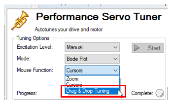
a. Drag and Drop Tuning - Overview

What if system performance is still not good enough? Examples. Too much:

• Position oscillation or overshoot at end of move
• Motor audible noise
• Speed variation
• Vibration on the load
• Motor shaft vibration when at standstill

The PST’s Drag & Drop Tuning feature allows offline simulation of the performance of different servo tuning settings right on the Bode plot. This is accomplished  by dragging and dropping  various gain/filter values in the Simulated Closed and Open Loop plots. The new values can then be loaded in the drive for an actual machine test.           

         Check the  Simulated plots:     

The goal of drag and drop tuning is to work toward the Optimal plot criteria. Procedure for doing drag and drop tuning:

• Place drive to the appropriate opmode (position or velocity mode)
• Slide VL.KP and make sure the closed loop plot is at 0 dB with no peaking and the open loop cross over occurs at the same point.    
• Slide the forward loop and feedback loop filters to the left or right to reduce any peaking to 0 dB or below.
• Adjust VL.KI to assure lower frequencies reach 0 dB without peaking
• If still need to increase performance switch to another filter type. Other filter types may lead to higher performance. Lead-Lag is typically used when high frequency performance is needed.

b. Drag and Drop Tuning - Example

For reference here is a bode plot meeting the main criteria for a good plot (and good machine performance). It is from the “ideal” load. Most application will not have a plot this good due to resonances (multi-body systems) and compliance. Yet you do not need to have a plot this good just need to meet the aforementioned criteria.

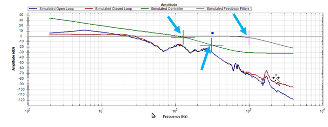
To use drag and drop tuning, hover over and you can see what parameter can be affected by that specific crosshair. There will be an X-plane and Y-plane on many that are individually adjustable by left mouse clicking and dragging up or down h the horizontal line or vertical line left or right. Hover over it and you will see the label appear. Example: 3 drag and drop “plus”  points shown):

Here is a plot in which the load has a resonance point at 70 Hz. This will result in unstable operation:

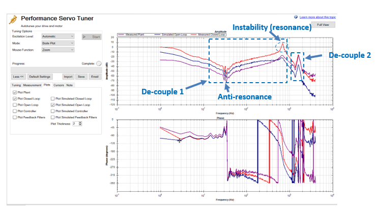
Reading this plot

•  The closed loop has a resonance above 0 dB. (Not good)
• This is a large system based on the anti-resonance at a low frequency of ~ 12 Hz.
• It is basically a multi-body system – two separate de-couplings
• Conclusion: More tuning is required

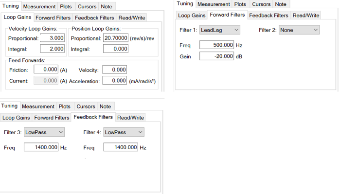
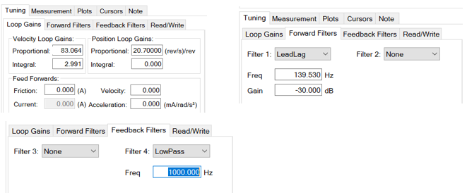
Tuning parameters settings for this plot:                      

                       

Using Drag and Drop tuning, the tuning was improved to this:
                    

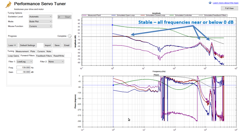
 The new gains are:

 

            

     

To verify the drag and drop simulation, a new Bode Plot is run on the physical system and provided similar results to the drag and drop simulation:

Comparing the gains

       

                          

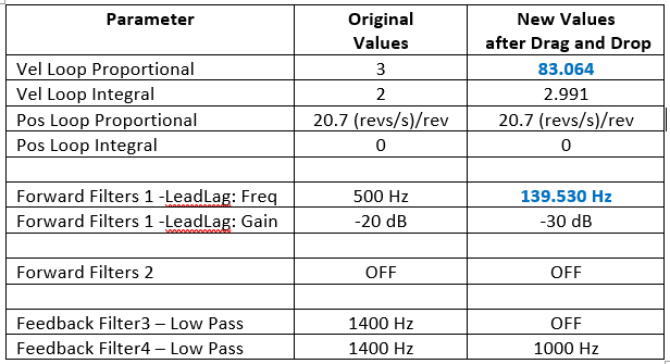
With Velocity Loop Proportional change of 3 to 83.064 and Forward Filter 1 change from 500 to 139.530 the BW of the system was increased considerably.

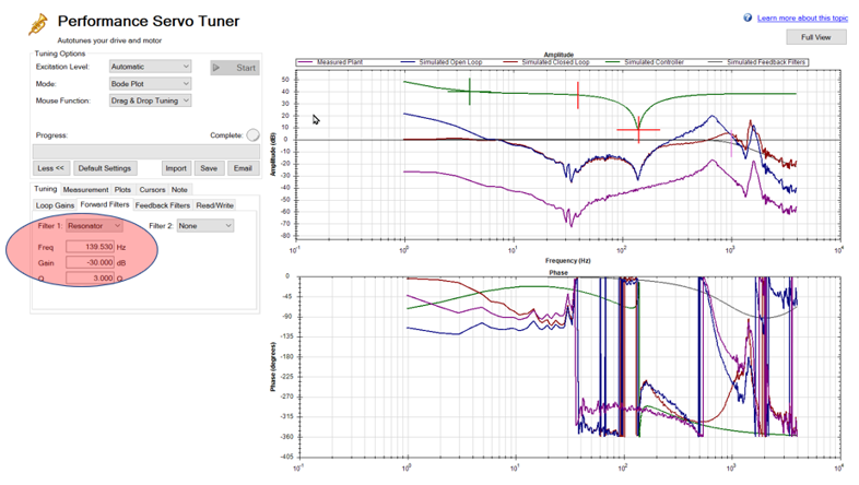
c. Wat if a different filter type was used?  

Sometimes performance can be improved by trying another filter. In this example what if the  filter type was changed from Lead-Lag to Resonator.  A Resonator can boast or reduce the gain and width at specific frequencies that results in increase overall machine performance.

Note: Optional filtering is available in the AKD. The AKD consists of 4 Bi-Quadratic filters, abbreviated BiQuad. This means that these filters with the use of their variables can create low pass, high pass, lead-lag, resonators, notch or peaking filters depending on your needs. Cascading them can also create custom effects. The custom filter option uses the Q, damping factor, and frequency information to create the variables within the mathematic calculations.

 

Here are the results when a Resonator filter was used with the same gains:

           

Filter overview

An overview of the 4 available filter types( abbreviated BiQuad) is as follow:

• LeadLag: The Leadlag filter is the default and will work for most servo systems.
• Lowpass: A Lowpass filter requires the least amount of processing time. The PST will place the Low Pass to get the maximum BW possible.
• Resonator: The Resonator filter is like a Notch filter with tunable BW and notch depth. The Resonator takes longer to calculate than the Leadlag filter.
• Custom: The Custom filter takes the longest to calculate and does not restrict the PST to a filter shape. This filter type provides excellent results but may significantly slow your computer while the filter is calculated. Use this one when the others fail to provide the needed performance

 

Final Notes

• Using Drag and Drop Tuning, different filters can be experimented with, and stable tuning can be achieved using alternate methods.
• Downloading and writing these tuning parameters must be done with care. The system reading is only as good as the feedback. If an ancillary resonance is in the system where no feedback is seen, you could affect this, and a drastic instability issue could become evident. Always use caution when downloading simulation based tunings.
• How do you know if you have achieved the best tuning? That depends on how much you expect the load to change over time and how close you are to getting to a positive resonance and how loose are your manufacturing tolerance. If you know the inertia and compliance of your load will change then you may want to build in a higher safety margin by have larger GM and PM values. The further you are for instability the more stable your system. The tradeoff will be higher GM/PM values may mean lower performance (move time, speed accuracy) or lower BW in the application
• It is important to understand the relationship between a servo gain and the dB value. Example: you need to raise or  lower the gain at specific frequencies in the plot by 20dB. The formula is:

20*log(Gain)  = change in dB     or      Log(Gain)=dB/20

• Then a gain of 10 is needed to raise the point 20dB. A  gain of -10 is needed to lower the point 20 dB. A gain of 100 with raise the point by 40dB.  A gain of 1000 will raise the point by 60dB. 3dB is 3/20 or 0.15. That being the log, the gain needed will be 10^0.14 or 1.42. Conclusion: multiply your present gain by 1.42 to get to zero dB if you are presently at -3dB

 

4. For More Information

        Tips and Tricks for the AKD Performance Servo Tuner: https://www.kollmorgen.com/en-us/developer-network/tips-and-tricks-akd-performance-servo-tuner/

        Bode plot Interpretation and Use.pdf  (attachment)

        Frequency Domain Training - The Use of the Bode Plot.pdf (attachment)

        Using Bode Plots to Improve Performance.pdf  (attachment)

       KOL-Auto-Tuning-WP-04-11-vSEO  (attachment)

       Using the Performance Servo Tuner Using the Performance Servo Tuner (kollmorgen.com)

       Using the Performance Servo Tuner: Advanced: Using the Performance Servo Tuner: Advanced (kollmorgen.com)